A language for pictures

The original PLAI course used arithmetic to introduce some ideas. On polling, students seemed more inclined towards picking something more interesting like picture composition. So we’ll take that track. I hasten to add that there’ll be additional work involved and less scaffolding, though you’ll be well rewarded by exposure to the process of building an understanding of a domain through language construction, from ground up, in addition to working through programming language principles. I will try to retain the spirit of the PLAI course through this exercise so that you can follow the concepts via the arithmetic route and still be able to relate to what we’re doing here.

Note

We’re not going to be building an “image processing toolkit”. What we’re interested in is making (hopefully) pretty pictures. The former is about processing images typically captured by cameras or scanners as a 2D array of “pixels”. The latter is about composing pictures, including but not limited to the “2D pixel array” variety.

Growing a language

We’re about to launch off a precipice in our efforts to figure out a language for composing pictures. When we set out on such a task in any domain, there are a few things we need to do to build up our understanding of the domain first. For what are you going to build a language for if you don’t understand it in the first place? We’ll need to –

1. Get a sense of the “vocabulary” we want for working with pictures.

2. Get a sense of how we wish to be able to generate pictures, transform them or combine more than one to form a new picture.

3. Figure out the essence of picture composition – i.e. a minimal “core language” in which we we can express the ideas we’re interested in. Translate more specific ideas into this core language.

Note that we do not need to get all of this right at the first shot. We can take some reasonable steps and improve what we have at hand when we recognize the opportunity. To do that effectively, we’ll need to keep our eye on the mentioned “minimal core” as we go along.

Credits

This section is named in honour of an amazing talk of the same title by Guy Steele, the co-creator of Scheme - Growing a language, by Guy Steele (youtube link) given in 1998. It is a fantastic talk and a great performance & delivery, that I much recommend students watch and contemplate on. The beginning of the talk may unfortunately put off some as it appears sexist, but Guy is aware of it and explains himself a little into the talk. So do press on.

A plausible vocabulary

Let’s consider 3 categories of images that students gave examples of –

1. “Primitives” such as discs, rectangles, squares and triangles. We include images loaded from files in this category since they do not depend on the content of other images. We’ll use the Plain PPM file format since it is a simple text-based format that’s easy to parse and write. [1]

2. Transformations – including colour transformations and spatial transformations like translation, rotation, scaling and mirroring. These take one image and modify their appearance to produce another “transformed” image.

3. Combinations – including placing one image on top of another, “blending” two images and such.

The above is already giving us a plausible vocabulary for talking about pictures to begin with, even though we don’t yet know what exactly a “picture” is. We can represent these ideas using s-expressions like below –

[1]

You’ve already been given instructions to write functions to read and write this format.

Primitives

(disc <radius>)
(square <width>)
(rectangle <width> <height>)
(image-from-file <filename.ppm>)

Transformations

(invert-colour <img>)
(gray-scale <img>)
(translate <dx> <dy> <img>)
(rotate <angle> <img>)
(scale <xscale> <yscale> <img>)

Combinations

(place-on-top <img1> <img2>)
(mask <mask-img> <img>)
(blend <img1> <img2>)

What some of them do might be obvious while others may not be so obvious. This means we’ll now need to commit to some “representation” of pictures so we can figure out these details.

In particular we need to understand “colour” first.

What is “colour”?

I’m not talking about a general perceptual understanding of colour here, though that is a fascinating topic worthy of its own course. For our purposes, we’ll satisfy ourselves with determing colour in terms of three well known colour components – red, green and blue. We’ll represent a mixture of these colour components by giving three real numbers in the range \([0.0,1.0]\) that given the proportions in which to mix them to get a colour. We’ll also use an “alpha” value in the range \([0.0,1.0]\) to indicate the opacity of a colour. This will be useful when we blend two colours. In typical image files as well as displays, these proportions are not usually represented as floating point numbers, for efficiency. They’re given as integers in the range \([0,255]\), with the assumption that we’ll scale them to \(255\) (or \(256\) which is close enough) to get the proportions.

We can represent such a colour easily in Racket using –

; The four colour components are floating point numbers
; in the range [0.0,1.0]
(struct colour (a r g b))

Once defined in this way, we can make a colour using (colour a r g b) and get the various components of a colour c using (colour-r c), (colour-b c) etc.

So, what is an “image” or “picture”?

When we look at a picture, what are we actually looking at? If we take up a magnifying glass in our hands, we can pore over the details of the picture by moving it over the region of interest to us. That is, we can consider for the moment that a picture is a mapping from a pair of spatial coordinates to a colour.

In the previous session on “lambda”, we represented whole numbers using functions to build up confidence that functions are powerful enough to capture all of computation. We should therefore expect that they will suffice for images too. Below, we’ll use Haskell type notation which you’re familiar with to capture the idea of the types of things we’re dealing with.

type Coords = (Float, Float)
type Image = Coords -> Colour

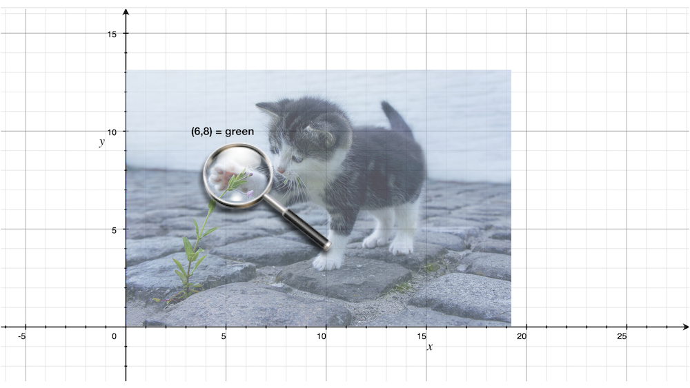
Fig. 1 An image can be thought of as a mapping from a pair of spatial coordinates \((x,y)\) to a colour value. (Credits: catpic and magglass)

Is it too abstract to think of a picture like that? Since we haven’t yet figured out how exactly we want to treat pictures, this is a reasonable starting point since we can produce a “raster image” (a 2D array of pixels) by calling the “image function” for various values of \(x\) and \(y\) and recording the colour produced.

Let’s now consider some simple pictures –

; disc :: Float -> Image
;
; Produces a white disc against a black background.
; The background is totally transparent everywhere outside
; the radius of the disc.
(define (disc radius)
    (λ (x y)
       (let ([r (sqrt (+ (* x x) (* y y)))])
         (if (< r radius)
             (colour 1.0 1.0 1.0 1.0)
             (colour 0.0 0.0 0.0 0.0)))))

; square :: Float -> Image
;
; (square 1.0) will make a unit square centered around
; the origin. Similar colour structure to the disc.
(define (square width)
    (λ (x y)
       (let ([half (* 0.5 width)])
           (if (and (> x (- half)) (< x half)
                    (> y (- half)) (< y half))
               (colour 1.0 1.0 1.0 1.0)
               (colour 0.0 0.0 0.0 0.0)))))

We can also write functions that transform these primitives spatially and in colour –

; translate :: Float -> Float -> Image -> Image
;
; Translates the given image by the given delta values in X and Y directions.
(define (translate dx dy img)
    (λ (x y)
       (img (- x dx) (- y dy))))

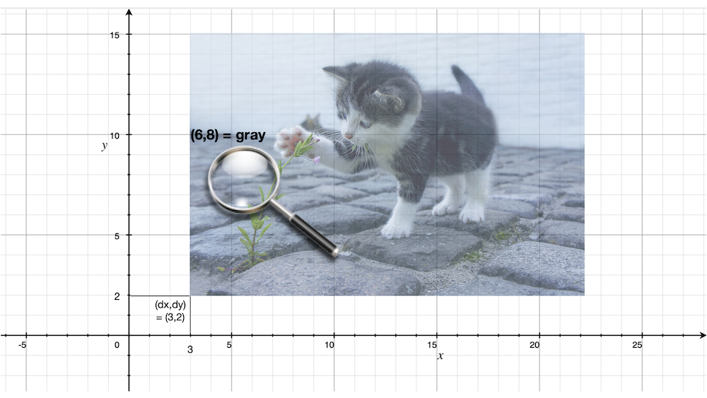
Fig. 2 The same cat picture above translated by \((3,2)\). The colour we’re now looking at at \((6,8)\) is at \((3,6)\) relative to the bottom left corner of the cat picture.

; scale :: Float -> Float -> Image -> Image
;
; (scale 0.5 0.5 <img>) will result in an image
; that's half the size in both x and y dimensions.
(define (scale xscale yscale img)
   (λ (x y)
      (let ([x2 (/ x xscale)]
            [y2 (/ y yscale)])
        (img x2 y2))))

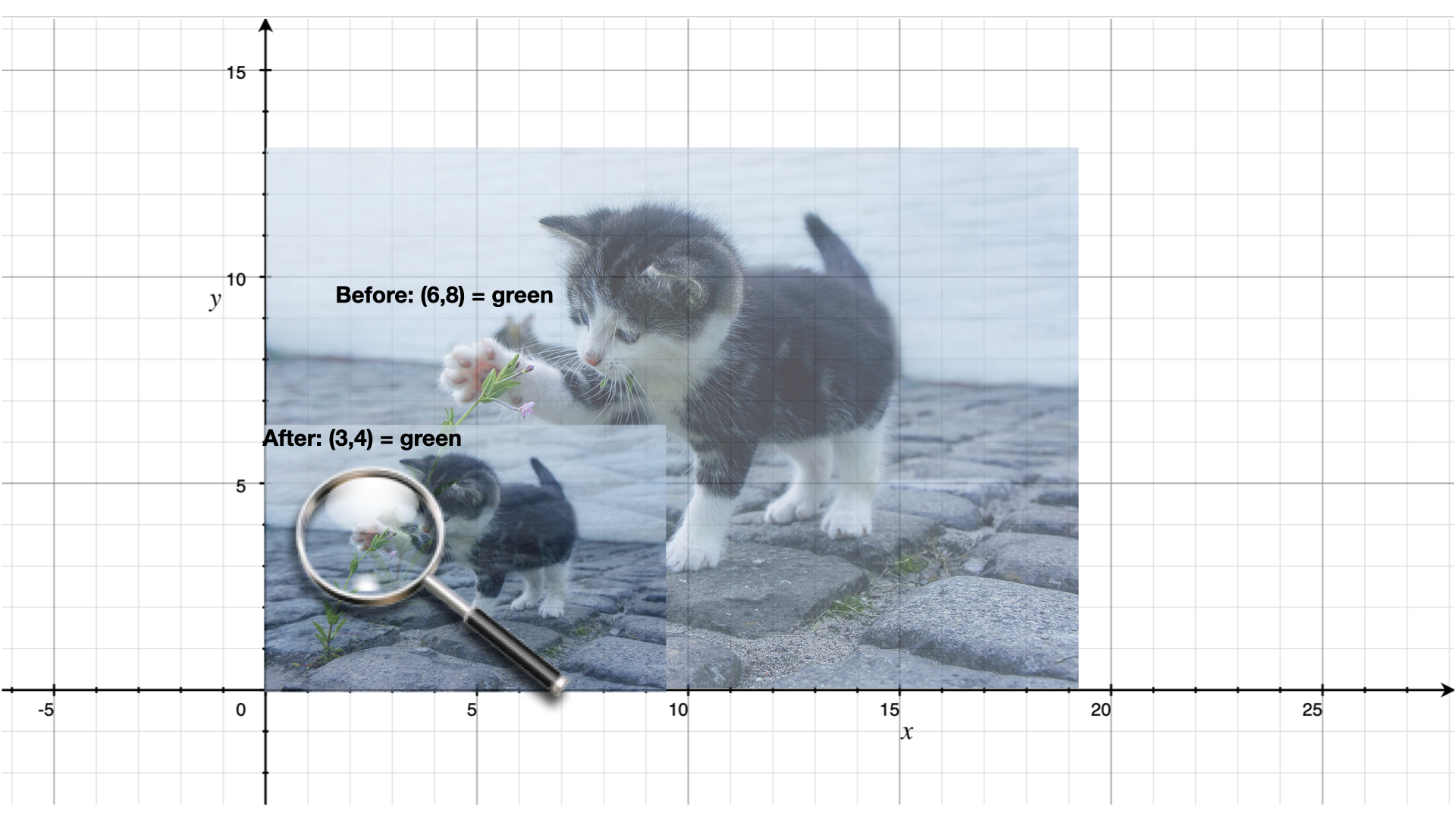
Fig. 3 The same cat picture above scaled by \((0.5,0.5)\). The colour we’re looking at when we look at \((3,4)\) in the result image is the same colour we get when we looked at \((6,8)\) in the original image.

Notice that though our scaling factors are \((0.5,0.5)\), we need to use the inverse of the scaling factors when figuring out which point in the original image we should look at.

Exercise

Implement the rotation function along similar lines. Hint: Recall the rotation matrix from your linear algebra course.

We’ll do a simple colour inversion before we go any further.

; invert-colour :: Image -> Image
;
; Note that we preserve the alpha as is so that opaque colours
; in the original are mapped to opaque but inverted colours in
; the transformed picture.
(define (invert-colour img)
    (λ (x y)
       (let ([c (img x y)])
         (colour (colour-a c)
                 (- 1.0 (colour-r c))
                 (- 1.0 (colour-g c))
                 (- 1.0 (colour-b c))))))

Composing transformations as functions

We now have a mini language at hand. Using the functions we’ve defined above, we can combine them to make new images. For example, (translate 5 5 (rotate 30 (square 2.0))). The expression (square 2.0) produces an image function that represents a square of width \(2.0\), which we rotate around the origin by \(30\) degrees and then translate it by \((5,5)\).

A first step to making an interpreter

We now consider what if we don’t evaluate that expression as a Scheme expression, but treat it as a program by quoting it – i.e. '(translate 5 5 (rotate 30 (square 2.0))). To dissect that, what we really have are three types of “picture expressions” –

1. (square <width>) which should produce a square.

2. (rotate <angle> <picture-expression>) which should rotate the specified picture.

3. (translate <dx> <dy> <picture-expression>) which should move the specified picture.

Notice that these picture expressions can also consist of other picture expressions and hence the possibility of composition.

The racket/match library provides a match macro that makes it easy for us to write an interpreter for such expressions.

#lang racket
(require racket/match)

; Our interpreter takes a "picture expression" and computes a picture
; by interpreting the instructions in it. Since these expressions can
; themselves contain other picture expressions, the interpreter is
; invoked recursively to compute them.
(define interpret-v1
    (λ (picexpr)
       (match picexpr
         [(list 'square width) (square width)]
         [(list 'rotate angle picexpr2) (rotate angle (interpret-v1 picexpr2))]
         [(list 'translate dx dy picexpr3) (translate dx dy (interpret-v1 picexpr3))]
         [_ (raise-argument-error 'interpret-v1 "Picture expression" picexpr)])))

In this case, we’ve used certain words like square and translate to express some concepts in our “language” and mapped these concepts to implementations specified in our “host language”, which is racket. In terminology, the “meaning” we give to these words is captured in our implementations. This “meaning” is referred to as “semantics”. The structure of the expressions that we use to denote this meaning is referred to as “syntax”.

Observe that the interpreter is recursive since the expressions that it works with are recursively specified. We can now use the above interpreter to compute our expression like this -

(define program '(translate 5.0 5.0 (rotate 30.0 (square 2.0))))
(interpret-v1 program)

Exercise

Read the documentation for match in the Racket docs to understand how the pattern is being specified in the code above. In particular, lists can be matched using the list constructor based expression. Quoted symbols will be matched literally and unquoted symbols will be taken as variables to be bound to the values in the corresponding slots in the list.

Once you’ve written the read-image and write-image functions in your assignment, you’ll be able to run the above interpreter to do some simple things with them. In the next section, we’ll look into what would make for a “core language” versus “surface syntax”.

An alternative representation

We represented the “program” as simply an s-expression. Our program in this case consisted of a single expression which our interpret “evaluated”. More typically when working on programming languages, the sub-expressions we used are given their own data structure and a tree is made by composing these sub-expressions. The tree is referred to as the “abstract syntax tree” as it captures the syntactic structure of the program, leaving aside (i.e. absracting) the sequence of characters from which it s constructed.

To capture the spirit of that, we can also represent our image primitives and transformations as structures like below –

(struct Disc (radius))
(struct Translate (dx dy picexpr))
(struct Rotate (deg picexpr))
; etc.

(define (picexpr? e)
   (or (Disc? e)
       (Translate? e)
       (Rotate? e)
       ; ...
       ))

We can then represent our program as an expression using the struct constructors as – (Translate dx dy (Rotate deg (Disc radius))). Note that this is not quoted, which means that the value which Scheme will compute when given this expression is a tree of sub-expressions. We can interpret this tree as follows -

(define interpret-v2
    (λ (picexpr)
       (match picexpr
          [(Disc radius) (disc radius)]
          [(Translate dx dy picexpr) (translate dx dy (interpret-v2 picexpr))]
          [(Rotate deg picexpr) (rotate deg (interpret-v2 picexpr))]
          [_ (raise-argument-error 'interpret-v2 "Picture expression as node" picexpr)])))

match lets you use the constructor names of struct declarations to deconstruct them and extract the parts. When you’re writing your own or extending the interpreter, remember that the tree is not made of pictures, but expressions that stand for pictures. These expressions will need to be interpreted to give them their meanings as pictures, hence the recursive calls to transform these sub-expressions to pictures that we can then compose.

Why bother?

We already had good enough functions that we can make use of to construct pictures. Why would we bother to make such an “interpreter” that so blatantly uses the same functions to do the same thing?

One part of the answer is that we’re trying to understand programming languages through the construction of such interpreters.

The second part is the process that we went through here. We modelled a domain using plain functions to understand what we’re building first. We then turned the kinds of expressions we wish to construct into an “abstract syntax tree” and built an “interpreter” to build what we want. Even if we do not build a full fledged programming language and stop here, we’ve done a powerful and highly under-used program transformation or “refactoring” technique called “defunctionalization”. It is called so because we took what’s initially a set of functions and turned calculations using those functions into a pure data structure – the AST. The advantage of this is that this AST can now be stored on mass media and transmitted over networks, which most host languages will not let you do with ordinary functions, especially if they have variables they close over.

We’re however going to go further than defunctionalization and build “proper” programming ability into our image synthesizer.

There’s still one more aspect. Our functions do not fully capture what we know about these operators. In particular, they do not capture some algebraic properties of these operators when they’re used together. For example, the expression (Translate 2 3 (Translate 20 30 (Disc 25))) is expected to produce the same picture as (Translate 20 30 (Translate 2 3 (Disc 25))) which in turn produces the same picture as (Translate 22 33 (Disc 25)).

So we can write an independent “program transformation function” that encodes this knowledge like this –

(define (rewrite picexpr)
   (match picexpr
     [(Translate dx1 dy1 (Translate dx2 dy2 picexpr))
      (rewrite (Translate (+ dx1 dx2) (+ dy1 dy2) picexpr))]
     [(Scale xscale yscale picexpr) (Scale xscale yscale (rewrite picexpr))]
     ; ... and so on for other untouched expressions.
     [_ picexpr]))

This function rewrite will precalculate a sequence of given translations as a single translation, which should give us some boost in efficiency given our underlying representation. Such transformation to code is done in most programming languages, working on the underlying “intermediate representation” (typically abbreviated IR) to perform various optimizations before generating the target machine code from the IR.